ESSAY / 2026

From Quantum Tunneling to Qubits: An Introduction to Quantum Computing

Developments in computer science and the need to process extremely huge amounts of data on a daily basis, increasingly calls for better processing power and hardware. However there is a limit to how small computer chips can get, until new challenges need to be addressed. Therefore computer science has to step into the realm of quantum mechanics. Although quantum computers are powerful tools for overcoming some challenges of big data processing, they are completely different from classical computers and not a substitute for them.

New methods and techniques are developed to implement the basics of quantum computing. This article will discuss the challenges regarding classical computers, the definition of quantum computation, the key differences between classical and quantum computers, definition of quantum bits or qubits, quantum gates and mathematical representation of them and how they work, and some methods of implementing quantum computers along with examples.

1. Introduction

Moore’s law states that the number of transistors on a microchip doubles every two years, while the cost is reduced.[1] This requires smaller and smaller transistors in computer processors. However, the transistors cannot get indefinitely small. Atomic level transistors face completely new challenges such as quantum tunneling, which can lead to current leakage. In recent years we have been witnessing a deviation from the trend of Moore’s law, as it seems to no longer be valid. On the other hand, information explosion, big data analysis and problems which involve too many variables require new and more efficient processing methods. Therefore, these challenges have increased interest in the development of such quantum computers.


Quantum computers are quite powerful in certain areas and for specific types of calculations, they are nevertheless not replacements for classical computers. Classical computers are good with solving complex calculations. Quantum computers, in contrast, are efficient in solving mass linear problems, such as linear equations, cryptography and encryption, search algorithms, weather forecast, and needless to say, quantum mechanical simulations.[2]


While classical computers use classical bits, which can take the value of either ‘0’ or ‘1’, quantum computers use quantum bits, or rather ‘qubits’ and use quantum gates to do calculations. Scientists have spent decades studying how to realize and implement qubits, quantum gates, and quantum computers. A few techniques and methods have been developed over the years. Despite being mostly in research and development phase, commercially built quantum computers are already out there in the market, the economical and energy costs and preparation time of which are still relatively high and the number of qubits is limited.


2. Classical and quantum computation comparison


Using classical computers for everyday tasks such as entertainment, multimedia and communication is quite trivial. Quantum computers cannot replace their classical counterparts in every field, where not only do they fail to increase efficiency when solving certain problems, but also can be really inconvenient. In the classical realm, the smallest unit for storing data is a bit, which can take discrete values of either zero or one (based on a present voltage). Then diodes, transistors, switches, etc. are used to implement logic gates (such as NOT, OR, and so on) in order to do logical operations on the binary inputs. Based on computational needs, different algorithms are used to do the calculation.


Qubits are the fundamental units of quantum information.[3] In the world of quantum mechanics qubits can not only take values of ‘0’ and ‘1’, but also a state of superposition of these values, with different coefficients for each state. Quantum gates are the quantum mechanical counterparts of classical logic gates. Since quantum computers can actually use states of quantum superposition to do calculations, therefore they can do some sort of computations with a lot less effort and in a much shorter time. For instance, breaking a simple classical encryption that could take days for a normal computer could be done by a quantum computer rather quickly. On the other hand quantum computers can be used to create strong cryptographic algorithms.[4]


Quantum computers also show a lot of potential in solving weather forecast problems, quantum search, quantum simulation, data mining and machine learning and much more. A lot of problems that quantum computers tackle are either practically near impossible to solve using classical computers, or extremely difficult and time consuming.

3. Josephson junction


One really important phenomenon in quantum mechanics is quantum tunneling, in which, when a quantum object, such as a subatomic particle, faces a barrier of finite potential, the probability of the object passing the barrier does not suddenly drop to zero at the boundary, but rather there is a chance that the quantum object passes through the barrier and simply exists on the other side, even if E<Vmax. Fig. 1 shows this interesting phenomenon, which makes possible much of our modern electronics.[5]
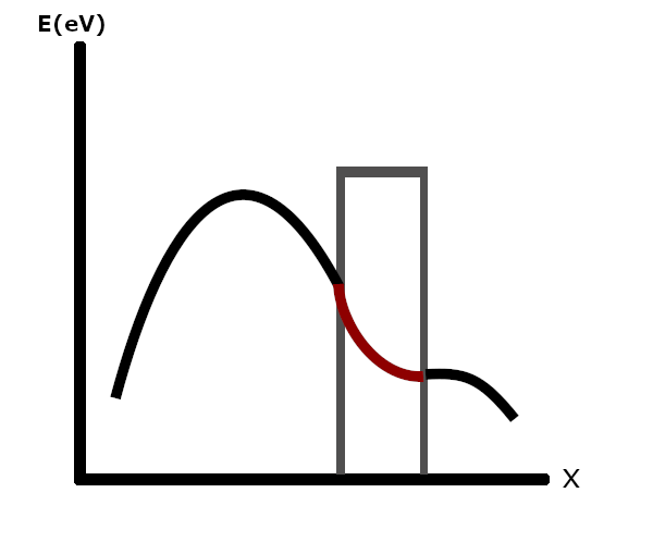
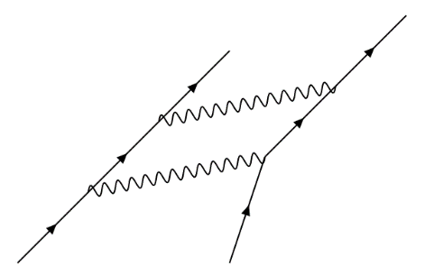
Fig. 1. Tunneling effect.

In superconductors that are cooled down to temperatures near absolute zero, half-spin electrons in pairs form whole spin quasi-particles that are condensed to a bosonic state. These so-called ‘Cooper pairs’ are all in the same state, and can be described as a constant wave function, or rather one complex number with an amplitude and a phase. This is the basic theory behind the flow of super-current in superconductors (see Fig. 2).

Fig. 2. A Feynman diagram illustrating the interaction between two electrons (straight lines) through phonons. The wiggly lines represent phonons, not photons.
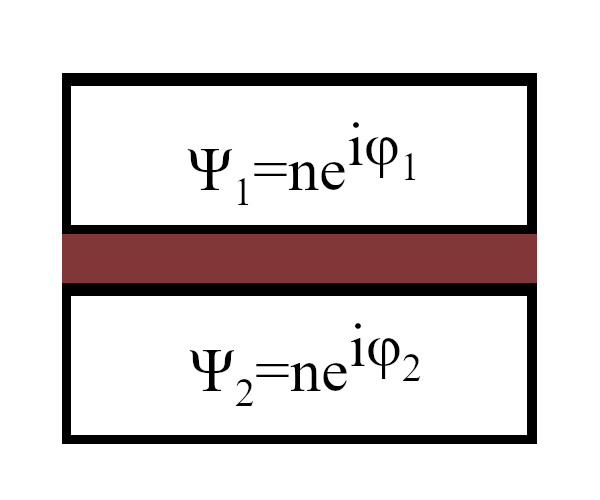
Fig. 2. A Feynman diagram illustrating the interaction between two electrons (straight lines) through phonons.

The wiggly lines represent phonons, not photons.


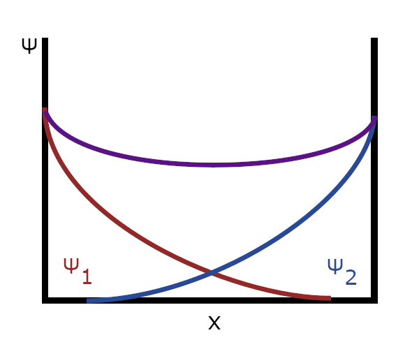
If we consider two pieces of superconductors like shown in Fig. 3, each with its own wave function, with a small barrier, which can be vacuum, an insulator or a piece of semiconductor, in between, we might initially think that the probability of electrons tunneling from one superconductor, over the barrier to the other is low; however Josephson suggested that there is a high probability of super-current passing through, without affecting the quasi-particle distribution.[6] The reason is that the wave function of Cooper pairs overlap if they are close enough, and add up to a single wave function over the barrier (see Fig. 4).

Fig. 3. Two superconductors separated by a dielectric.

As mentioned earlier, each piece of superconductor is in its own phase, so there is a phase difference ΔΦ over the barrier. Since phases can be added or subtracted, the phase difference is represented by just Φ as

\[ \Phi = \phi_2 - \phi_1 \ \tag{3.1} \]


with a super-current that is related to the critical current Jc, with a phase difference of \(\frac{\pi}{2}\) after which there is a voltage across the junction with the current density[7]

\[ J_s = J_c \sin(\Phi) \tag{3.2} \]


and with a voltage across the barrier that is dependent on the time derivative of Φ and is defined as[8]

\[ U(t)=\frac{\hbar}{2e}\frac{\partial \Phi}{\partial t} \tag{3.3} \]

and these relations are known as Josephson’s first and second relation respectively.

Fig. 4. Overlapping of wave functions over the barrier.

The phase difference gives rise to non-linearity in the voltage-current relation, which is an important feature of Josephson junctions. Josephson junction is really important in designing superconducting qubits.

4. Qubit


Qubits are the fundamental units of quantum information. As mentioned earlier, qubits can be in a superposition state, and that is the key point that defines the differences between classical computers and quantum computers.

Since we want the qubits to have the values one, zero or a state of superposition of both, theoretically properties of many subatomic particles can be used as qubits. For instance polarization of a photon, or spin of an electron, or even spin of nuclei of atoms can be used as qubits.

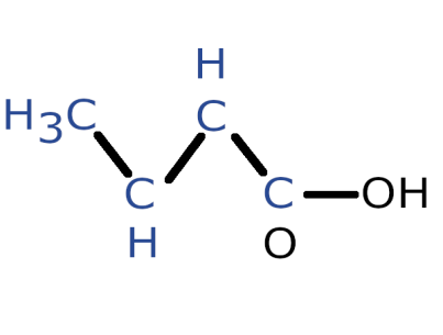
One easy but rather limited way of creating qubits is to use the spin of fermionic nuclei and a nuclear magnetic resonance spectroscopy machine.[9] For this method half-spin nuclei, also known as fermionic nuclei such as 1H, 13C, 15N, 19F or 31P are used. This method is for research purposes only, and has huge limitations, such as the number of qubits, and liquid state related issues, which fall outside the scope of this article. Also most authors believe that it will not be possible to build NMR quantum computers large enough to solve real computational problems. However, very basic classic problems of quantum computing, such as Deutsch’s algorithm have been implemented using NMR-based quantum computers. Fig. 5 shows propionic acid, which has been used to implement NMR quantum computing.

Fig. 5. Propionic acid is one of the substances that has been used to implement NMR quantum computing. Qubits are marked in blue. All H atoms in the methyl group are used as a single logical qubit.
Fig. 5. Propionic acid is one of the substances that has been used to implement NMR quantum computing.
Qubits are marked in blue. All H atoms in the methyl group are used as a single logical qubit.

Although photons could be useful in the field of quantum cryptography, the usage of photons is not discussed in quantum computation. The why deserves its own dedicated piece, and while important, a detailed discussion again exceeds the goals of this article.

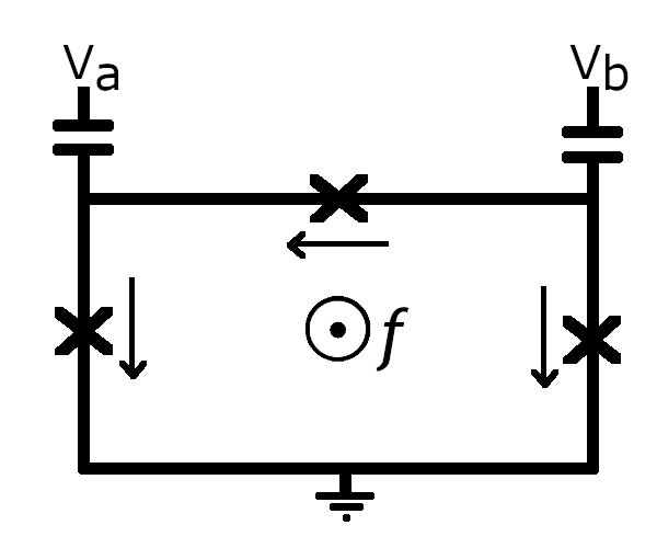
Superconducting quantum computing consists of a series of state of the art methods of creating qubits and quantum computers. Flux qubits, also known as superconducting persistent current qubits, like shown in Fig. 6, are micrometer sized loops of superconducting material that include Josephson junctions.[10] These flux qubits are usually made on silicon or sapphire wafers using vapor deposition or electron beam lithography. One common method of creating such loops is to use shadow evaporation technique, in which masks are held above the substrate during the deposition, and deposition happens at different angles.

Fig. 6. Schematics of a three junction qubit. Arrows show the direction of current flow. The magnetic flux is sticking out of the page.
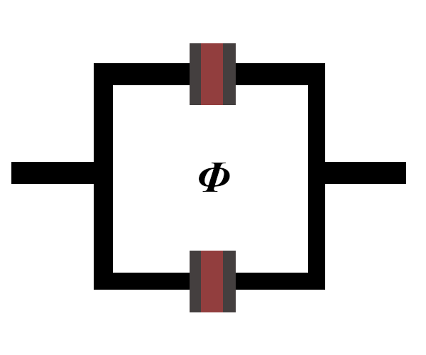
Fig. 6. Schematics of a three junction qubit. Arrows show the direction of current flow.

The magnetic flux is sticking out of the page.


Flux qubits consist of three Josephson junctions, and use circulating microcurrents of opposite signs as their two states. The flux in the two states can be detected with a superconducting quantum interference device or SQUID, and the states can be manipulated with magnetic fields. A SQUID, like (see Fig. 7), is a very sensitive magnetometer used to measure extremely subtle and weak magnetic fields, based on superconducting loops containing Josephson junctions.

Fig. 7. Simplified schematic of a superconducting quantum interference device or SQUID. In this figure Φ is flux.
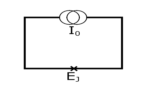
Fig. 7. Simplified schematic of a superconducting quantum interference device or SQUID. In this figure Φ is flux.


If in the loop of a SQUID there were neither junctions nor were external magnetic fields present, what would normally happen is that the current would be divided in half, and go through both branches of the loop. However the presence of an external magnetic field establishes a phase difference and induces a change in the current, and thus one branch will have higher current passing through, which pushes the total current of that branch to a value higher than the critical current of the Josephson junction, thus there will be flow of super-current over the junction. But we know from Maxwell’s equation, that we need a changing magnetic flux for it to be able to induce any current. However, if the magnetic flux is more than half the magnetic flux quantum or Φ0 , then it will push current until flux is an integer multiple of magnetic flux quanta. In contrast, if the flux is less than half the magnetic flux quantum, then it will reduce it to zero. This is also a governing rule in flux qubits.

Another type of superconducting qubit that includes Josephson junctions is phase qubit, which is based on superconductor-insulator-superconductor (S-I-S) Josephson Junctions, in which, like shown in Fig. 8, Josephson junction with energy parameter EJ is biased by a current I0.

Fig. 8. Phase qubit.

A charge qubit is also another Josephson junction-based qubit, which uses charge states as its basis states. Transmon qubit is an example of a charge qubit. The main difference between all the previously mentioned superconducting qubits is the ratio of Josephson energy to charging energy.

Mathematically, qubits can be represented as orthonormal basis vectors. For instance

\[ \lvert 0 \rangle = \begin{bmatrix} 1 \\ 0 \end{bmatrix} \tag{4.1}\ \]


And

\[ \lvert 1 \rangle = \begin{bmatrix} 0 \\ 1 \end{bmatrix} \tag{4.2} \]


as the two states. Thus the distinct states of two qubit quantum registers can be represented as

\[ \lvert 00 \rangle = \begin{bmatrix} 1\\0\\0\\0 \end{bmatrix}, \quad \lvert 01 \rangle = \begin{bmatrix} 0\\1\\0\\0 \end{bmatrix}, \quad \lvert 10 \rangle = \begin{bmatrix} 0\\0\\1\\0 \end{bmatrix}, \quad \lvert 11 \rangle = \begin{bmatrix} 0\\0\\0\\1 \end{bmatrix} \tag{4.3} \]

And of course qubits can be in superposition of both states

\[ \lvert \psi \rangle = a\lvert 0 \rangle + b\lvert 1 \rangle \tag{4.4} \]


with a and b being amplitudes (\(|a|^2 + |b|^2 = 1\)). In general, qubits can be represented as vectors in Bloch spheres where

\[ \lvert \psi \rangle = \cos\left(\frac{\theta}{2}\right)\lvert 0 \rangle + e^{i\phi}\sin\left(\frac{\theta}{2}\right)\lvert 1 \rangle \tag{4.5} \]

And operations on qubits can be defined as certain rotations.

5. Quantum gates


Quantum gates are the quantum mechanical descriptions of classical logic gates. They are used to design and create quantum circuits operating on qubits. Mathematically quantum logic gates are linear operators, acting on orthonormal qubit vectors, and are commonly represented by matrices.

Table 1 shows some quantum logic gate symbols.[11] Having the initial state of the qubit, after applying gate operators, we can easily find new states of qubits just by following the gates and instructions step by step. That is different from finding quantum mechanical eigenstates, for which one has to solve the Schrödinger equation.

Table 1. Quantum logic gates.
OperatorGate
Pauli-X (X) or NOTPauli-X GateorNOT Gate
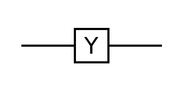
Pauli-Y (Y)Pauly Y-Gate
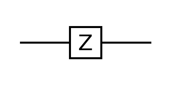
Pauli-Z (Z)Pauly Z-Gate
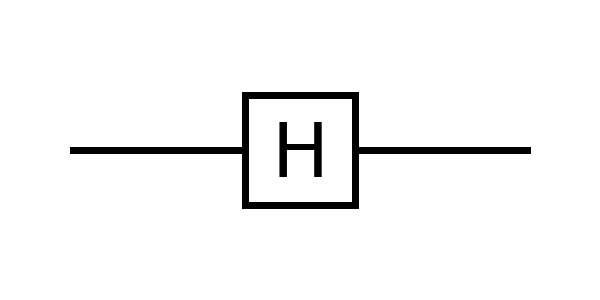
HadamardHadamard Gate
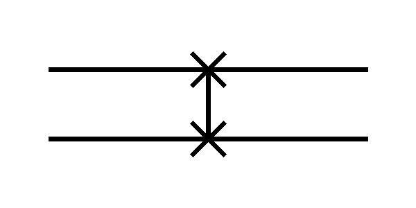
SwapSwap Gate
Controlled-NOT (CNOT)Controlled Not (CNOT) Gate

Applying gates, and therefore operators on qubits is analogous to rotation of state vectors in a Bloch sphere.

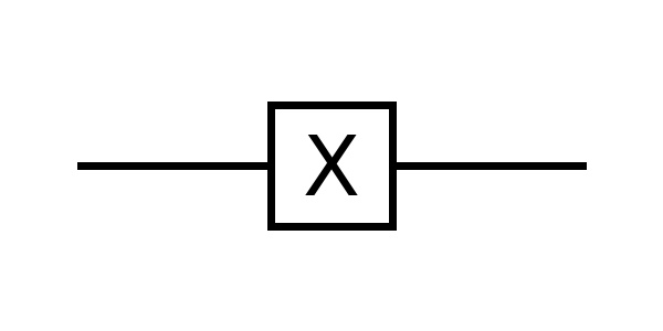
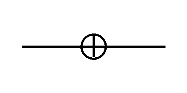
Pauli gate is the most basic gate in quantum computing, and it is the same as Pauli spin matrix in quantum mechanics. Pauli X gate, which is the same as NOT gate, rotates the state vector of qubits 180° around the x-axis. Matrix representation of this gate is the same as Pauli’s σx matrix and is defined as

\[ X = \begin{bmatrix} 0 & 1 \\ 1 & 0 \end{bmatrix} \tag{5.1} \]

and the Y-gate is defined as a 180° rotation around the y-axis of the Bloch sphere. The matrix representation of this gate is

\[ Y = \begin{bmatrix} 0 & -i \\ i & 0 \end{bmatrix} \tag{5.2} \]


and finally Z gate, which represents a 180° rotation around the z-axis is defined as

\[ Z = \begin{bmatrix} 1 & 0 \\ 0 & -1 \end{bmatrix} \tag{5.3} \]


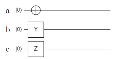
Fig. 9 shows each of these gates acting on 3 different |0⟩ qubits. In Fig. 9 (a) X gate is denoted by NOT gate symbol. If we operate an X gate on a |0⟩ qubit, we notice that the qubit flips, and the probability of finding the qubit to be in the new state of |1⟩ is now 1; based on

\[ \begin{bmatrix} 0 & 1 \\ 1 & 0 \end{bmatrix} \begin{bmatrix} 1 \\ 0 \end{bmatrix} = \begin{bmatrix} 0 \\ 1 \end{bmatrix} \]


and respectively for Y gate

\[ \begin{bmatrix} 0 & -i \\ i & 0 \end{bmatrix} \begin{bmatrix} 1 \\ 0 \end{bmatrix} = \begin{bmatrix} 0 \\ i \end{bmatrix} = i \begin{bmatrix} 0 \\ 1 \end{bmatrix} \]


in which the qubit flips. However, the difference with the NOT gate is the negative imaginary number coefficient Finally, in case of Z gate we have

\[ \begin{bmatrix} 1 & 0 \\ 0 & -1 \end{bmatrix} \begin{bmatrix} 1 \\ 0 \end{bmatrix} = \begin{bmatrix} 1 \\ 0 \end{bmatrix} \]

which does nothing to the qubit in this example, but combined with other gates, it will have its own effects.

Fig. 9. Pauli gates. (a) X gate (here represented as NOT gate instead of X) operating on a qubit. (b) Y gate operating on a qubit. (c) Z gate operating on a qubit.

Fig. 9. Pauli gates. (a) X gate (here represented as NOT gate instead of X) operating on a qubit. (b) Y gate operating on a qubit. (c) Z gate operating on a qubit.


Probably the most important quantum logic gate is the Hadamard gate. Matrix representation of the Hadamard gate is[12]

\[ H = \frac{1}{\sqrt{2}}\begin{bmatrix} 1 & 1 \\ 1 & -1 \end{bmatrix} \tag{5.4} \]


and it is analogous to a 180° rotation around the z-axis followed by a 90° rotation around the y-axis. The most interesting property of the Hadamard gate is that it can take a basis state as an input, and output a superposed state and vice versa. Fig. 10. shows this gate being applied to both basis qubits.
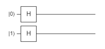
Fig. 10. Hadamard gate being applied to both basis vectors.

If we operate the Hadamard transform on a |1⟩ qubit we will have

\[ \frac{1}{\sqrt{2}} \begin{bmatrix} 1 & 1 \\ 1 & -1 \end{bmatrix} \begin{bmatrix} 0 \\ 1 \end{bmatrix} = \frac{1}{\sqrt{2}} \begin{bmatrix} 1 \\ 0 \end{bmatrix} - \frac{1}{\sqrt{2}} \begin{bmatrix} 0 \\ 1 \end{bmatrix} \]


which is a superposed state of both basis states, and has equal probability of outputting either |0⟩ or |1⟩ upon measurement. Similarly applying this transform to a |0⟩ qubit will return

\[ \frac{1}{\sqrt{2}} \begin{bmatrix} 1 & 1 \\ 1 & -1 \end{bmatrix} \begin{bmatrix} 1 \\ 0 \end{bmatrix} = \frac{1}{\sqrt{2}} \begin{bmatrix} 1 \\ 0 \end{bmatrix} + \frac{1}{\sqrt{2}} \begin{bmatrix} 0 \\ 1 \end{bmatrix} \]


which is also a superposition of both basis qubits. In terms of Dirac notation, the Hadamard gate can be denoted by

\[ H = \frac{1}{\sqrt{2}}\left[(\lvert 0\rangle+\lvert 1\rangle)\langle 0\rvert+(\lvert 0\rangle-\lvert 1\rangle)\langle 1\rvert\right] \tag{5.5} \]

and by applying this operator to both basis qubits we will have

\[ H\lvert 0\rangle = \frac{\lvert 0\rangle+\lvert 1\rangle}{\sqrt{2}} \tag{5.6} \]


\[ H\lvert 1\rangle = \frac{\lvert 0\rangle-\lvert 1\rangle}{\sqrt{2}} \tag{5.7} \]


which are superposed states with equal probabilities of measuring each basis state. In these examples the probabilities of finding the qubits to be in state |0⟩ are

\[ \left|\langle 0 | H | 0 \rangle\right|^2 = \left| \frac{\langle 0|0\rangle + \langle 0|1\rangle}{\sqrt{2}} \right|^2 = \frac{1}{2} \]


\[ \left|\langle 0 | H | 1 \rangle\right|^2 = \left| \frac{\langle 0|0\rangle - \langle 0|1\rangle}{\sqrt{2}} \right|^2 = \frac{1}{2} \]


and also, it is worth mentioning that the Hermitian conjugate of the Hadamard operator is the Hadamard operator itself


\[ H = H^\dagger \tag{5.8} \]


and since

\[ HH^\dagger = I \tag{5.9} \]


if we apply the Hadamard gate to a qubit two times in a row, it will act as identity operator and leave the qubit completely unchanged, given that we do not hit the qubit with other operators between the two Hadamards. For instance

\[ H(H|1\rangle) = H\left( \frac{|0\rangle-|1\rangle}{\sqrt{2}} \right) \]


which is equal to

\[ \frac{1}{\sqrt{2}} \left( \frac{|0\rangle+|1\rangle}{\sqrt{2}} - \frac{|0\rangle-|1\rangle}{\sqrt{2}} \right) \]


thus gives us

\[ \frac{|0\rangle+|1\rangle-|0\rangle+|1\rangle}{2} = |1\rangle \]


and for an initially superposed qubit condition could be written

\[ H\left( H\frac{|0\rangle+|1\rangle}{\sqrt{2}} \right) = H\left( \frac{ \frac{|0\rangle+|1\rangle}{\sqrt{2}} + \frac{|0\rangle-|1\rangle}{\sqrt{2}} }{\sqrt{2}} \right) \]


then we have

\[ \frac{2H|0\rangle}{2} = H|0\rangle = \frac{|0\rangle+|1\rangle}{\sqrt{2}} \]


which is again the same as the identity operator acting on the superposed qubit.

Swap gate is another common and useful logic gate in quantum computation. The operator corresponds to the matrix

\[ \operatorname{SWAP} = \begin{bmatrix} 1 & 0 & 0 & 0\\ 0 & 0 & 1 & 0\\ 0 & 1 & 0 & 0\\ 0 & 0 & 0 & 1 \end{bmatrix} \tag{5.10}\]


and takes as input two separate qubits and swaps them like


\[ \begin{aligned} \operatorname{SWAP}|00\rangle &= |00\rangle,\\ \operatorname{SWAP}|01\rangle &= |10\rangle,\\ \operatorname{SWAP}|10\rangle &= |01\rangle,\\ \operatorname{SWAP}|11\rangle &= |11\rangle. \end{aligned} \]


For instance a swapped |01⟩ qubit would be

\[ \begin{bmatrix} 1 & 0 & 0 & 0\\ 0 & 0 & 1 & 0\\ 0 & 1 & 0 & 0\\ 0 & 0 & 0 & 1 \end{bmatrix} \begin{bmatrix} 0\\ 1\\ 0\\ 0 \end{bmatrix} = \begin{bmatrix} 0\\ 0\\ 1\\ 0 \end{bmatrix} \]

which is equal to |10⟩.

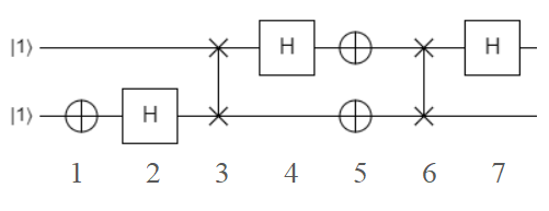
As an example of the above gates, the problem in Fig. 11 is given. In order to figure out the final state of each given qubit, we should follow the logic gates on one until we reach a swap gate, after which we should make a break, backtrack and follow the other path to the swap gate. Then we can swap the states and continue the solution on either qubit paths.

Fig. 11. An example of some basic gates being applied on two qubits.

Starting with the second qubit, we first encounter a NOT gate at step 1, which gives the state |0⟩. Then the Hadamard results in a superposed state. At step 3 we have a swap gate. If we backtrack the first qubit we will have |1⟩ for the second qubit and a state of superposition for the first. Continuing with the second, we have a NOT gate at step 5, which leaves us with |0⟩. At step 6 we have another swap gate. We can stop and trace back the state of the first qubit. At step 3, after the swap, we have a superposition. Another Hadamard gate at step 4 of the first qubit after step 2 of the second qubit gives back the basis state of |0⟩.

Note that the swap just interchanges the states of the qubits. It looks as though the Hadamards are being applied successively. At step 5 we have again |1⟩. At step 6 we swap |1⟩ state of the first qubit with |0⟩ of the second and run it through the final Hadamard gate to have yet another superposition of states. Thus, the final state would be \(\frac{|0\rangle + |1\rangle}{\sqrt{2}}\) for the first and |1⟩ for the second qubit. Therefore, probability of measuring the qubits to be in state |1⟩ for the first and the second qubit is \(\frac{1}{2}\) and 1 respectively.

A controlled gate is another type of gate with multiple qubits as inputs. Controlled gates normally take one qubit as a control input, and consider its state, and do operations on other input qubits based on the state of the control qubit at input. Controlled-NOT gate, or rather CNOT, is probably the most famous one of the controlled gates. This gate acts on two qubits, and applies a NOT or X operator on the second one, if the first qubit, or rather the control qubit, should be in state |1⟩. The matrix description of CNOT operator is

\[ \operatorname{CNOT} = \begin{bmatrix} 1 & 0 & 0 & 0\\ 0 & 1 & 0 & 0\\ 0 & 0 & 0 & 1\\ 0 & 0 & 1 & 0 \end{bmatrix} \tag{5.11} \]


and it represents the mapping \(|x,y\rangle \xrightarrow{\operatorname{CNOT}} |x,y\oplus x\rangle\). For instance, for the input state of |11⟩ we have

\[ \begin{bmatrix} 1 & 0 & 0 & 0\\ 0 & 1 & 0 & 0\\ 0 & 0 & 0 & 1\\ 0 & 0 & 1 & 0 \end{bmatrix} \begin{bmatrix} 0\\ 0\\ 0\\ 1 \end{bmatrix} = \begin{bmatrix} 0\\ 0\\ 1\\ 0 \end{bmatrix} = |10\rangle \]


which is equal to the state |10⟩. One interesting circuit that contains both the CNOT gate and the Hadamard gate is the entangler circuit (see Fig. 12). Starting with two qubits in two basis states, we can put them in an entangled state, if we run the control qubit first through the Hadamard gate, and then apply the CNOT gate. So, starting with a random state like |00⟩ we have

\[ \left(\operatorname{CNOT}\right)\left(H_1\right)|00\rangle \]


after applying the Hadamard gate we get

\[ \operatorname{CNOT} \left( \frac{|00\rangle+|10\rangle}{\sqrt{2}} \right) \]


which is not an entangled state yet. After CNOT operates on this superposed state we will have

\[ \operatorname{CNOT} \left( \frac{|00\rangle+|10\rangle}{\sqrt{2}} \right) = \frac{|00\rangle+|11\rangle}{\sqrt{2}} \]

which is a state of entanglement. Therefore, if we make a measurement on the first qubit, and find out that it is in the state |1⟩, then without measurement, we know with probability of 1 that the second qubit has the state |1⟩, even though the initial probability of finding each qubit in either states before measurement was \(\frac{1}{2}\).
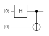
Fig. 12. The Hadamard and CNOT gates being applied on two qubits in order to entangle their states.

Just in a similar way, the CNOT gate can operate on entangled states to detangle them, so

\[ \operatorname{CNOT} \left( \frac{|00\rangle+|11\rangle}{\sqrt{2}} \right) = \frac{|00\rangle+|10\rangle}{\sqrt{2}} \]


gives

\[ \frac{|00\rangle+|10\rangle}{\sqrt{2}} = \frac{|0\rangle+|1\rangle}{\sqrt{2}} \otimes |0\rangle \]


which is not an entangled state anymore. In this example we started with two |0⟩ qubits, and got a state of entanglement, in which both final qubits were in the same state. However, note that if we start with a state of |11⟩, we end up having

\[ \frac{|01\rangle - |10\rangle}{\sqrt{2}} \]


in which the qubits have opposite states. In general, if our control qubit has an initial state of |1⟩, then we end up with two entangled qubits with opposite states, and in case of beginning with control qubit being in state |0⟩, then both qubits will be in the same state after entanglement. However, we can use a Pauli-X gate, or a NOT gate to flip one qubit, and get the other type of entanglement (see Fig. 13). As an example, given that we start with |00⟩, after entanglement we will end up with

\[ \frac{|00\rangle - |11\rangle}{\sqrt{2}} \]


and after passing the first qubit through a NOT gate we will have

\[ \frac{|10\rangle - |01\rangle}{\sqrt{2}} \]
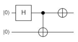

in which the two qubits have opposite states.

Fig. 13. NOT gate operating on one qubit after entanglement results in another state of entanglement.

Fig. 13. NOT gate operating on one qubit after entanglement results in another state of entanglement.


6. Quantum algorithms


In analogy to classical algorithms, quantum algorithms are sets of instructions to be run step by step on quantum computers. They are meant to solve problems and do certain tasks in a much more efficient way, or with less effort and much faster. Some examples of quantum algorithms are:[13]  Grover’s algorithm, which finds with a probability of greater than half a specific item within a randomly ordered database of N items using order of \(\sqrt{N}\) operations, Bernstein and Vazirani algorithm, which is based on the earlier work of Deutsch and Jozsa[14], and Shor’s algorithm, which solves integer factorization problems.

6.1. Deutsch’s algorithm


Deutsch’s problem is one of classic quantum computer problems, that shows how quantum computers are able to solve certain problems in less time, and in less cycles than classical computers. Consider the Boolean function f, which does the mapping \(\{0,1\} \xrightarrow{f} \{0,1\}\). There are four functions with such property: two constant functions


\[ f(0) = f(1) = 0 \quad \text{and} \quad f(0) = f(1) = 1 \tag{6.1.1} \]


and two balanced functions


\[ f(0) = \tilde{f}(1) = 0 \quad \text{and} \quad f(0) = \tilde{f}(1) = 1 \tag{6.1.2} \]


In David Deutsch’s problem, the observer is allowed to evaluate the function not more than just once, and needs to deduce from the outcome, not the value of the function f, but rather whether it is constant or balanced.[15] Classically, one needs to run the function twice for both inputs 1 and 0 to make a decision. We define the Hermitian operator f-controlled-NOT, which does the mapping


\[ |x,y\rangle \xrightarrow{f\text{-}c\text{-}N} |x, y \oplus f(x)\rangle \tag{6.1.3} \]


Note that this operator is quite similar to controlled-NOT gate, the only difference being \(y \oplus f(x)\) in the mapping.


The inputs to the system are two qubits, with the state \(\frac{1}{\sqrt{2}}\left(|00\rangle - |01\rangle\right)\). The second qubit can be thought of as a |1⟩ qubit that has been acted on by a Hadamard operator, which leaves it in a state of superposition. For simplicity, we can leave out the normalization factors. As shown in Fig. 14, we run the first qubit through a Hadamard gate to get the state


\[ |\psi\rangle = \frac{1}{2} \left( |00\rangle + |10\rangle - |01\rangle - |11\rangle \right) \tag{6.1.4} \]


which is a state of superposition of all four possible inputs.
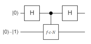

Fig. 14. Simplified diagram of Deutsch’s algorithm.

Fig. 14. Simplified diagram of Deutsch’s algorithm.


Then we proceed by applying the f-controlled-Not on the state |𝜓⟩. Therefore, for each \(x \in \{0,1\}\) we have


\[ U_f\left[|x\rangle\left(|0\rangle-|1\rangle\right)\right] = |x\rangle \left( |0\oplus f(x)\rangle - |1\oplus f(x)\rangle \right) \tag{6.1.5} \]


which is


\[ = (-1)^{f(x)} |x\rangle \left( |0\rangle-|1\rangle \right) \tag{6.1.6} \]


thus, by adding in the values for x we get


\[ \left[ (-1)^{f(0)}|0\rangle + (-1)^{f(1)}|1\rangle \right] \left( |0\rangle-|1\rangle \right) \tag{6.1.7} \]


which can be written as


\[ (-1)^{f(0)} \left( |0\rangle + (-1)^{f(0)\oplus f(1)} |1\rangle \right) \left( |0\rangle-|1\rangle \right). \tag{6.1.8} \]


After applying the final Hadamard gate we have the state


\[ (-1)^{f(0)} \left| f(0)\oplus f(1) \right\rangle \tag{6.1.9} \]


which means that if the first qubit comes out to be in the state |0⟩, then the function f is constant and otherwise, f is balanced.


This is possible, thanks to superposition, which is the magical quantum mechanical property that lets us see the outcome of running the qubits through a gate in one cycle instead of two.


This basic algorithm can be generalized. Many other quantum computing algorithms are based on Deutsch’s algorithm. This is just a basic example of how quantum computers can reduce the number of cycles needed to solve a problem, by using quantum mechanical phenomena, such as superposition and entanglement. Although this example did not use entangled states at all, you should be able to see how this phenomenon can also reduce the steps needed in quantum data processing in a similar way.


Conclusion


Quantum computers might not be a big part of our daily lives now, and it might take years until we see them everywhere; nevertheless they are useful tools, based on the basic rules of quantum mechanics, to solve a series of problems, which are time and energy consuming for conventional computers to handle, much easier and faster.


Nobody claims that quantum computers are going to be substitutions for classical computers, desktops, or servers, as they are not only expensive, difficult to make and work with, huge in size, and power consuming. They are also not the most efficient in solving many problems, which classical computers handle easily. In the years to come still entertainment systems, desktop and office computers, servers, mobiles and many more devices will still be based on classical computation with classical bits. However, we will see more and more quantum computers, with less energy consumption and more qubits, which translates to more quantum processing power. Different sub-branches of science have tried to provide methods of implementing quantum computation, such as NMR quantum computation, solid state methods and superconducting quantum computation.


Implementing most quantum computers currently requires usage of cryogenics, such as liquid nitrogen and helium, in order to achieve temperatures near absolute zero, to be able to see the quantum effects and phenomena. This makes the process of creating quantum computers and stabilizing them costly and energy consuming. In addition, quantum computers are susceptible to a lot of noise from outside, or even potentially inside. Thermal noise, noise from ions, and electromagnetic noise can be mentioned as only some challenges that scientists need to overcome.


Throughout the years, the subject of quantum computers has been extensively studied by top scientists, and many methods and techniques have been developed in order to realize this idea. Different quantum properties can be used as states of quantum bits or qubits, such as polarization of photons, spin of subatomic particles, or even energy or current of Josephson junctions. For instance, we can use the spin of Fermionic nuclei in the NMR method, or the current passing through the loops of Flux qubits as basis qubits.


Qubits are different from conventional bits, in that they can be in a superposed state. This is the key idea behind the whole concept of quantum computers.


Quantum gates are equivalents of classical logic gates. Just as logic gates in classical computers are used to design and create circuits, which operate on bits and process data, quantum gates serve the purpose of processing qubits. They can mathematically be represented as matrices and operators. One can implement different circuits and algorithms using quantum gates, and if the states of qubits are known in the beginning it is not required to solving any differential equations for figuring out any eigenstates. It just takes following the chronological paths of quantum gates and applying the operators in the right order to find out the final state of qubits.


Quantum algorithms, in analogy to classical computer algorithms, are sets of instructions to be run on quantum computers, in order to do calculation. The goal of these quantum algorithms is to solve time consuming, or certain complex problems in less orders of time, or with less effort using quantum computers. Deutsch’s algorithm is one of the oldest, most basic and most popular algorithms that goes to show how quantum computers can solve a black-box problem in less cycles and therefore less time than classical computers. There are also other examples of quantum algorithms available, such as Grover’s algorithm, Bernstein and Vazirani algorithm, Shor’s algorithm, and many more.


Quantum computers have applications in a variety of fields, such as medical science and pharmacy, search, data mining, machine learning and artificial intelligence, security, encryption and cryptography, weather forecast, mathematics and quantum simulations.


Although quantum computers are currently mostly a big topic for research, and they are indeed used mostly for that goal, commercial quantum computers have been developed, and are available. They work based on the basic concepts mentioned in this article, and bring users new methods of solving some problems, which were sometimes near impossible up to this date. However, this is just the beginning of the quantum computing era, and there are yet a lot to be discovered and improved. One example is to increase the number of qubits, or to achieve quantum effects at room temperature, or make quantum computers much more stable and noise resistant. With all that in mind, it is not an overstatement to say that quantum computers are no longer just dreams, but rather the reality of today, and the days to come. Maybe one day soon they will be part of the daily lives of people, just like classical computers.


Acknowledgment


This article is a review of the work of other great scientists, with the goal of gathering the most useful basic nuggets of information about quantum computing for beginners in one place. Any errors in the article are my own and should not tarnish the reputations of these esteemed persons, upon whose work I based this article.


References


[1] Moore, G. E. (1965). Cramming more components onto integrated circuits. 
[2] Boghosian, B. M., & Taylor IV, W. (1998). Simulating quantum mechanics on a quantum computer. Physica D: Nonlinear Phenomena, 120(1-2), 30-42.
[3] Schumacher, B. (1995). Quantum coding. Physical Review A, 51(4), 2738.
[4] Bernstein, D. J. (2009). Introduction to post-quantum cryptography. In Post-quantum cryptography (pp. 1-14). Springer, Berlin, Heidelberg.
[5] Griffiths, David J. (2017). Introduction to quantum mechanics. Cambridge University Press.
[6] Josephson, B. D. (1962). Possible new effects in superconductive tunneling. Phys. Lett, 1(7), 251.
[7] Josephson, B. D. (1965). Supercurrents through barriers. Advances in Physics, 14(56), 419-451.
[8] Josephson, B. D. (1974). The discovery of tunneling supercurrents. Reviews of Modern Physics, 46(2), 251.
[9] Jones, J. A. (2001). Quantum computing and nuclear magnetic resonance. PhysChemComm, 4(11), 49-56.
[10] Orlando, T. P., Mooij, J. E., Tian, L., Van Der Wal, C. H., Levitov, L. S., Lloyd, S., & Mazo, J. J. (1999). Superconducting persistent-current qubit. Physical Review B, 60(22), 15398.
[11] Barenco, A., Bennett, C. H., Cleve, R., DiVincenzo, D. P., Margolus, N., Shor, P., & Weinfurter, H. (1995). Elementary gates for quantum computation. Physical Review A, 52(5), 3457.
[12] Aharonov, D. (2003). A simple proof that Toffoli and Hadamard are quantum universal. arXiv preprint quant-ph/0301040.
[13] Coles, P. J., Eidenbenz, S., Pakin, S., Adedoyin, A., Ambrosiano, J., Anisimov, P., ... & Gunter, D. (2018). Quantum algorithm implementations for beginners. arXiv preprint arXiv:1804.03719.
[14] Deutsch, D., & Jozsa, R. (1992). Rapid solution of problems by quantum computation. Proceedings of the Royal Society of London. Series A: Mathematical and Physical Sciences, 439(1907), 553-558.
[15] Cleve, R., Ekert, A., Macchiavello, C., & Mosca, M. (1998). Quantum algorithms revisited. Proceedings of the Royal Society of London. Series A: Mathematical, Physical and Engineering Sciences, 454(1969), 339-354.